Python编程产生非均匀随机数的几种方法代码分享

1.反变换法

设需产生分布函数为F(x)的连续随机数X。若已有[0,1]区间均匀分布随机数R,则产生X的反变换公式为：

F(x)=r, 即x=F-1(r)

反函数存在条件：如果函数y=f(x)是定义域D上的单调函数,那么f(x)一定有反函数存在,且反函数一定是单调的。分布函数F(x)为是一个单调递增函数，所以其反函数存在。从直观意义上理解，因为r一一对应着x,而在[0,1]均匀分布随机数R≤r的概率P(R≤r)=r。 因此,连续随机数X≤x的概率P(X≤x)=P(R≤r)=r=F(x)

即X的分布函数为F(x)。

例子:下面的代码使用反变换法在区间[0, 6]上生成随机数，其概率密度近似为P(x)=e-x

import numpy as npimport matplotlib.pyplot as plt# probability distribution we're trying to calculatep = lambda x: np.exp(-x)# CDF of pCDF = lambda x: 1-np.exp(-x)# invert the CDFinvCDF = lambda x: -np.log(1-x)# domain limitsxmin = 0 # the lower limit of our domainxmax = 6 # the upper limit of our domain# range limitsrmin = CDF(xmin)rmax = CDF(xmax)N = 10000 # the total of samples we wish to generate# generate uniform samples in our range then invert the CDF# to get samples of our target distributionR = np.random.uniform(rmin, rmax, N)X = invCDF(R)# get the histogram infohinfo = np.histogram(X,100)# plot the histogramplt.hist(X,bins=100, label=u'Samples');# plot our (normalized) functionxvals=np.linspace(xmin, xmax, 1000)plt.plot(xvals, hinfo[0][0]*p(xvals), 'r', label=u'p(x)')# turn on the legendplt.legend()plt.show()

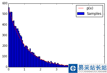
一般来说，直方图的外廓曲线接近于总体X的概率密度曲线。

2.舍选抽样法(Rejection Methold)

用反变换法生成随机数时，如果求不出F-1(x)的解析形式或者F(x)就没有解析形式，则可以用F-1(x)的近似公式代替。但是由于反函数计算量较大，有时也是很不适宜的。另一种方法是由Von Neumann提出的舍选抽样法。下图中曲线w(x)为概率密度函数，按该密度函数产生随机数的方法如下：

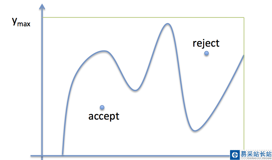
基本的rejection methold步骤如下：

1. Draw x uniformly from [xmin xmax]

2. Draw x uniformly from [0, ymax]

3. if y < w(x)，accept the sample, otherwise reject it

4. repeat

即落在曲线w(x)和X轴所围成区域内的点接受，落在该区域外的点舍弃。

例子:下面的代码使用basic rejection sampling methold在区间[0, 10]上生成随机数，其概率密度近似为P(x)=e-x

# -*- coding: utf-8 -*-'''The following code produces samples that follow the distribution P(x)=e^−x for x=[0, 10] and generates a histogram of the sampled distribution.'''import numpy as npimport matplotlib.pyplot as pltP = lambda x: np.exp(-x)# domain limitsxmin = 0 # the lower limit of our domainxmax = 10 # the upper limit of our domain# range limit (supremum) for yymax = 1N = 10000  # the total of samples we wish to generateaccepted = 0 # the number of accepted samplessamples = np.zeros(N)count = 0  # the total count of proposals# generation loopwhile (accepted < N):    # pick a uniform number on [xmin, xmax) (e.g. 0...10)  x = np.random.uniform(xmin, xmax)    # pick a uniform number on [0, ymax)  y = np.random.uniform(0,ymax)    # Do the accept/reject comparison  if y < P(x):    samples[accepted] = x    accepted += 1    count +=1  print count, accepted# get the histogram info# If bins is an int, it defines the number of equal-width bins in the given range (n, bins)= np.histogram(samples, bins=30) # Returns: n-The values of the histogram,n是直方图中柱子的高度# plot the histogramplt.hist(samples,bins=30,label=u'Samples')  # bins=30即直方图中有30根柱子# plot our (normalized) functionxvals=np.linspace(xmin, xmax, 1000)plt.plot(xvals, n[0]*P(xvals), 'r', label=u'P(x)')# turn on the legendplt.legend()plt.show()