Python数据拟合与广义线性回归算法学习

机器学习中的预测问题通常分为2类：回归与分类。

简单的说回归就是预测数值，而分类是给数据打上标签归类。

本文讲述如何用Python进行基本的数据拟合，以及如何对拟合结果的误差进行分析。

本例中使用一个2次函数加上随机的扰动来生成500个点，然后尝试用1、2、100次方的多项式对该数据进行拟合。

拟合的目的是使得根据训练数据能够拟合出一个多项式函数，这个函数能够很好的拟合现有数据，并且能对未知的数据进行预测。

代码如下：

import matplotlib.pyplot as plt import numpy as np import scipy as sp from scipy.stats import norm from sklearn.pipeline import Pipeline from sklearn.linear_model import LinearRegression from sklearn.preprocessing import PolynomialFeatures from sklearn import linear_model  ''''' 数据生成 ''' x = np.arange(0, 1, 0.002) y = norm.rvs(0, size=500, scale=0.1) y = y + x**2  ''''' 均方误差根 ''' def rmse(y_test, y):  return sp.sqrt(sp.mean((y_test - y) ** 2))  ''''' 与均值相比的优秀程度，介于[0~1]。0表示不如均值。1表示完美预测.这个版本的实现是参考scikit-learn官网文档 ''' def R2(y_test, y_true):  return 1 - ((y_test - y_true)**2).sum() / ((y_true - y_true.mean())**2).sum()   ''''' 这是Conway&White《机器学习使用案例解析》里的版本 ''' def R22(y_test, y_true):  y_mean = np.array(y_true)  y_mean[:] = y_mean.mean()  return 1 - rmse(y_test, y_true) / rmse(y_mean, y_true)   plt.scatter(x, y, s=5) degree = [1,2,100] y_test = [] y_test = np.array(y_test)   for d in degree:  clf = Pipeline([('poly', PolynomialFeatures(degree=d)),      ('linear', LinearRegression(fit_intercept=False))])  clf.fit(x[:, np.newaxis], y)  y_test = clf.predict(x[:, np.newaxis])   print(clf.named_steps['linear'].coef_)  print('rmse=%.2f, R2=%.2f, R22=%.2f, clf.score=%.2f' %   (rmse(y_test, y),   R2(y_test, y),   R22(y_test, y),   clf.score(x[:, np.newaxis], y)))     plt.plot(x, y_test, linewidth=2)   plt.grid() plt.legend(['1','2','100'], loc='upper left') plt.show() 

该程序运行的显示结果如下：

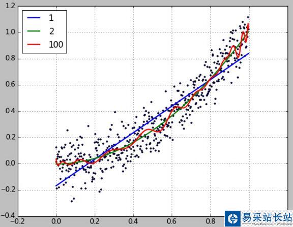
[-0.16140183  0.99268453]
rmse=0.13, R2=0.82, R22=0.58, clf.score=0.82
[ 0.00934527 -0.03591245  1.03065829]
rmse=0.11, R2=0.88, R22=0.66, clf.score=0.88
[  6.07130354e-02  -1.02247150e+00   6.66972089e+01  -1.85696012e+04
......
-9.43408707e+12  -9.78954604e+12  -9.99872105e+12  -1.00742526e+13
-1.00303296e+13  -9.88198843e+12  -9.64452002e+12  -9.33298267e+12
  -1.00580760e+12]
rmse=0.10, R2=0.89, R22=0.67, clf.score=0.89
显示出的coef_就是多项式参数。如1次拟合的结果为
y = 0.99268453x -0.16140183